Normal distribution curve and its main properties
Normal distribution curve >> Sample statistics distribution
Many phenomena and processes of our reality obey the normal law. For example, you are very likely to have average mental capacity ... well, plus or minus standard deviation.

Dembitskyi S. Normal distribution curve and its main properties [Electronic resource]. - Access mode: http://www.soc-research.info/quantitative_eng/1.html
Prior to talking about the specific methods used to collect and analyze quantitative data, it is necessary to consider the basic principles underlying the quantitative approach in general. These include: a) the use of properties of the normal distribution (or other distributions, chi-square, Fisher’s, Student’s, etc.); b) the use of peculiarities of sample statistics distribution; c) taking into account random errors that occur in any sample research.
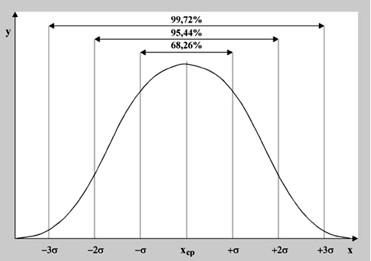
Any property under study has a corresponding distribution in the population. Very often, it is normal and is characterized by two parameters – mean and standard deviation. However, these two parameters differ from each other in an infinite set of normal curves. The mean sets the position of the curve on the number axis and acts as initial value. Standard deviation sets the width of this curve, it depends on the units of measurement and acts as the scale of measurement. Normal distribution curve (further – NDC) is a theoretical model representing fully symmetrical and smooth frequency distribution. It is bell-shaped, has one vertex, and its ends tend to infinity in both directions. The NDC’s main property is that the distance along the distribution abscissa (horizontal axis) measured in the units of standard deviation from the arithmetic mean always gives the same total area under the curve: between ± 1 standard deviation – 68.26% of the area, between ± 2 standard deviation – 95.44% of the area, between ± 3 standard deviation – 99.72% of the area. In fact, the area in this case is equivalent to the number of people with corresponding parameters in the population.
Any property under study has a corresponding distribution in the population. Very often, it is normal and is characterized by two parameters – mean and standard deviation. However, these two parameters differ from each other in an infinite set of normal curves. The mean sets the position of the curve on the number axis and acts as initial value. Standard deviation sets the width of this curve, it depends on the units of measurement and acts as the scale of measurement. Normal distribution curve (further – NDC) is a theoretical model representing fully symmetrical and smooth frequency distribution. It is bell-shaped, has one vertex, and its ends tend to infinity in both directions. The NDC’s main property is that the distance along the distribution abscissa (horizontal axis) measured in the units of standard deviation from the arithmetic mean always gives the same total area under the curve: between ± 1 standard deviation – 68.26% of the area, between ± 2 standard deviation – 95.44% of the area, between ± 3 standard deviation – 99.72% of the area. In fact, the area in this case is equivalent to the number of people with corresponding parameters in the population.
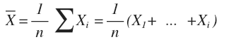
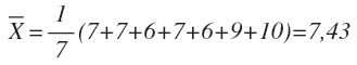
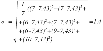
where Σ (Xi) is the sum of observation values, n is the number of observations. Let us calculate the arithmetic mean of the number of hours Ivan Petrov spent sleeping every day for the last week. As a week has seven days, n = 7. Xi is X1 = 7 hours (Monday), X2 = 7 hours (Tuesday), X3 = 6 hours (Wednesday), X4 = 7 hours (Thursday), X5 = 6 hours (Friday), X6 = hours (Saturday), X7 = 10 hours (Sunday). Thus,
Standard deviation is one of the most frequently used measures of dispersion (measures that characterize the heterogeneity of distribution). If, in our hypothetical example about Ivan Petrov, he slept for 8 hours every day, then no heterogeneity would be observed. In this case, the standard deviation would equal 0 (complete homogeneity of distribution).
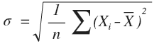
In our case, the standard deviation is equal to (see previous example):
Despite the fact that no empirical distribution’s form meets this ideal model, many of them are close enough to it, which allows us to assume them normal. This assumption, in its turn, allows us to use the NDC and its properties to analyze the corresponding empirical distributions.
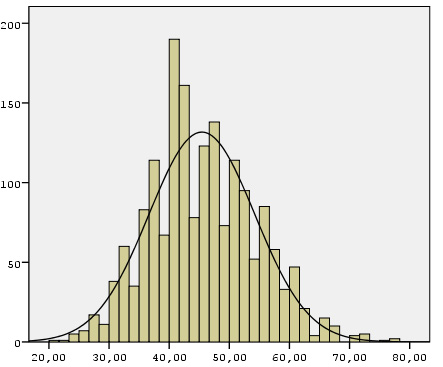
The above diagram illustrates the empirical distribution for the psychological feature of anxiety among respondents (n = 1725) reflecting the population of Ukraine (the survey was held in 2008). The graph shows both, empirical distribution, i.e. actual responses received (columns 20 to 80, where lower values correspond to lower anxiety, and higher values – to higher anxiety) and the ideal model of normal distribution (bell-curve). As the chart shows, empirical distribution does not match 100% of the ideal model of the NDC. Nevertheless, empirical distribution is close enough to normal, so we can use the properties of the latter. So, knowing that mean for respondents’ anxiety is 45, and standard deviation is 9, we can conclude that 68.26% of the population of Ukraine has the social well-being between 36 and 54 points. Due to the measurement error this information is rather approximate, but still close enough to the true values.
- default_titleХили Дж. Статистика. Социологические и маркетинговые исследования. - К.: ООО "ДиаСофтЮП"; СПб.: Питер, 2005. - 638 с.
- default_titleНаследов А. Математические методы психологического исследования. - СПб.: Речь, 2004. - 392 с.
- Show More