Information obtained from the sample is bound to the population by a mechanism called sample statistics distribution. Sample statistics distribution (further – SSD) is the theoretical distribution of statistics’ probabilities (by statistics we may mean, for example, the average value of a particular feature) for all possible samples of a given size. Thus, the SSD includes the value of all statistics corresponding to each possible combination of a given sample size. The most important feature of the SSD is that its characteristics are based on the laws of probability theory rather than on empirical information.
Example:
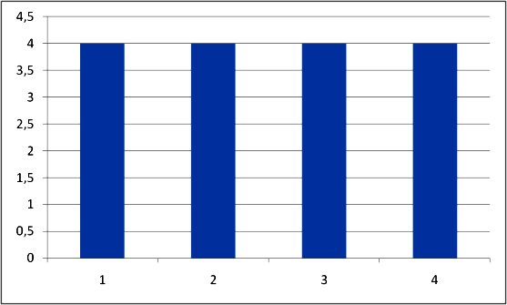
Let us assume that the population consists of only 16 people, and the sample we want to extract – of 3 people. The parameter to be estimated is the average number of rooms in the respondents’ flats. Let us assume that in the population 4 people have 1 room, 4 people – 2 rooms, 4 people – 3 rooms, and 4 people – 4 rooms. Such a distribution is called uniform and in this case looks as follows:

Accordingly, the first respondent selected into the sample can have a one-, two-, three- or four-room flat. The same is true for the second and third respondents. Knowing this, and applying the addition and multiplication rules for probabilities, we can calculate the probability of formation of a particular variant of the sample.

Addition rule for probabilities: when two events are mutually exclusive, the probability of either occurring is the sum of the probabilities of each event.
Multiplication rule for probabilities: the probability of any number of independent events occurring simultaneously is the product of their individual probabilities.
For more information on these rules we recommend referring to Gregory A. Kimble’s book “How to Use (And Misuse) Statistics”.

First, let us calculate the probability of obtaining three basic samples: A) all three respondents will have the same number of rooms; B) two respondents have the same number of rooms, and the third one has a different number; B) all three respondents have a different number of rooms.
Option A = 4/16 * 3/15 * 2/14 = 24/3360 or 0.7%;
Option B = 4/16 * 3/15 * 4/14 = 48/3360 or 1.4%;
Option C = 4/16 * 4/15 * 4/14 = 64/3360 or 1.9%.
Second, let us consider all possible combinations of samples with the size of three people for a given population. Different versions of these samples are grouped according to the average value of rooms they indicate (Mean).

Knowing the probability of basic samples (all of the presented combinations fall under one of the three options), and having a number of combinations corresponding to each of the possible means, we can calculate the probability of obtaining a particular mean for the sample of three people.
As an example, let us calculate the probability of obtaining a sample that would give a mean of 2 (№ 4 in the chart). This group has one sample of Option A (2+2+2), three samples of Option B (1+1+ 4, 1+4+1, 4+1+1) and six samples of Option C (2+1+3, 2+3+1, 1+3+2, 1+2+3, 3+2+1, 3+2+1). Now, based on the probability of formation of each option, we can obtain the total probability of X mean = 2:
1 * the probability of Option A + 3 * the probability of Option B + 6 * the probability of Option C = 0.7% * 1 + 1.4% * 3 + 1.9 * 6 = 0.7% + 4 2% + 11.4% = 16.3% (actually 16.4%, 0.1% is lost as a result of rounding). Likewise, we can calculate the probability of obtaining all other means for the sample of three people. The graph of the aforementioned information will look as follows:

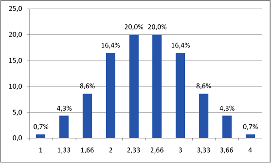
As you can see, the described distribution is very close to normal. This is an important point, which for the given SSD is expressed in the central limit theorem: given a distribution with mean μ and variance σ2, the sampling distribution of the mean approaches a normal distribution with mean μ and variance σ2/n, where n is the number of samples.
If to specify this theorem for our case, it is obvious that the probability of obtaining the sample with the mean close to the true mean (for our population of 16 people μ = 2,5) is much higher than the probability of obtaining the sample with the mean distant from the population mean. Thus, the probability of obtaining the sample whose mean minimally deviates from the true mean (by 0.17 or 0.16 points) is 40%. Then, the probability of obtaining the sample whose mean deviates from the true mean by no more than 0.5 points is 72.8%. Consequently, the probability of obtaining the sample whose mean deviates from the true mean by more than 0.5 points is 27.2%.
Of course, this example does not fully comply with the conditions of the central limit theorem due to the small size of both the population and the sample. However, it vividly demonstrates the specific character of the SSD and the peculiarities of its features for simple random sampling.
There are other cases of the SSD different from the normal distribution (e.g., Student’s distribution, Fisher’s, chi-square test, and others). However, the principle of their use is similar in nature – they allow us to estimate the probability of certain events and to make scientific conclusions on this basis.