Interval estimation
In many cases it may be necessary to estimate the corresponding parameter of the population on the basis of a single sample parameter (its mean or proportion). If the sample is large enough (over 100 observations), it is possible to calculate the interval where the true value will occur with a given probability, with the help of the properties of the normal distribution curve, as well as the central limit theorem.
As you may recall from Chapter II, the distribution of sample means is normal. Consequently, the probability of obtaining a sample with the mean close enough to the population mean is rather high. However, even when the sample mean is essentially different from the population mean, the confidence interval [in most cases] will include the true value. Only in very rare cases we may obtain the sample where the sample and population parameters are so different that the true value will not occur in the confidence interval.
We will not go into detail of the relevant evidence and examples, but will discuss the technique of calculating confidence intervals.
Confidence intervals for the means

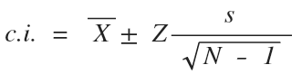
where Z is the standardized value determined by the alpha level or p-value (the probability that the true value will not occur in the confidence interval);
s – standard deviation for the sample;
n – sample size.
It is obvious that s and n are known from the study itself. In its turn, Z is determined using the chart of standardized values:

Confidence level indicates the probability of the true value occurring in the interval calculated.
Here is an example. Let us assume the sample (n = 300) tells us that the mean for monthly income for the citizens of Kiev is 4000 UAH, and the standard deviation is 75 UAH. If we are satisfied by the error probability of 5% (alpha – 0.05), then Z = ± 1,96.

Hence:

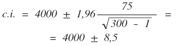
Thus, the true value for the citizens of Kiev must occur in the interval between 3991.5 UAH and 4008.5 UAH with 95% probability.
Confidence intervals for proportions

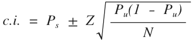
As compared with the previous one, this formula also includes sample size and Z-value. The latter is also determined using the chart above.
Other components include:
Ps – proportion value for the sample;
Pu – proportion value for the population.
The most attentive of you might wonder where to look for Pu if we want to use Ps for its estimation. Or if we know Pu, then why do we need Ps? Indeed, we only need Ps to estimate the unknown Pu. The way out of this situation is quite simple – we assume that Pu is the value (as you remember, for proportions it can vary from 0 to 1) that would give us the highest value of the expression of Pu (1-Pu). Then the confidence interval itself will have the highest value (all other conditions being equal / ceteris paribus). In fact, the researcher must deliberately increase the interval, since a longer interval is more likely to include the true value for the population we are trying to determine. This value is 0.5: 0.5 (1-0.5) = 0.5 * 0.5 = 0.25
Now here is an example. Let us assume that according to the results of the pre-election survey, 17% of the population are ready to vote for the oppositional party (Ps = 0,17), the sample size is 1,200 people, and the alpha level is 0.01.
Then:

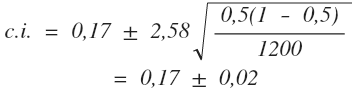
Consequently, from 15% to 19% of the population will vote for the oppositional party with 99% probability.