Statistical hypothesis testing
With statistical hypothesis testing, based on the data obtained, the researcher verifies the hypothesis stating that all determined relations between phenomena or differences between groups are the result of random errors.
Statistical hypothesis testing consists of the following steps: 1) Verifying assumptions. 2) Formulating statistical hypotheses. 3) Determining alpha level (p-value). 4) Calculating empirical test value and degrees of freedom. 5) Applying theoretical distribution: defining critical value and its comparison with empirical value.
Let us illustrate the basis of statistical hypothesis testing with the chi-square test for independence. This test determines whether there is a relationship between two variables, based on contingency tables. It is a nonparametric test, i.e. it does not require verifying assumptions about the form of distribution of sample statistics.
Step 1. To use the chi-square test, the data must meet only two assumptions:
a) Independent random samples are used. Independent samples occur when respondent selection for one sample does not affect respondent selection of another sample.
First, these data must be obtained from randomly selected students (for example, with the random selection from the list of all university students). In this case, the sample will also be independent – any male or female not yet in the sample can be further selected, no matter who was selected last.
b) Variables belong to a nominal scale. Since nominal scales are considered the "weakest", the use of ordinal and metric variables is also possible (after the number of their categories is reduced to the necessary amount).
For example, look at the table below, where the influence of students’ gender on their learning efficiency is tested:
Green represents the marginal frequencies in lines and columns. They will be needed later to calculate the expected frequencies.
| Efficiency | Gender |
Total
|
|
Female |
Male |
||
| Satisfactory (with D and/or E) | 16 |
12 |
28 |
| Good or Excellent (no D/E, only B/C/A) | 20 |
4 |
24 |
| Excellent (only A) | 10 |
0 |
10 |
| Total | 46 |
16 |
62 |
Step 2. Statistical hypotheses are divided into two types – null and alternative. Depending on the statistical method, the null hypothesis states either the absence of differences between groups (contrast of means or proportions) or the absence of relations between variables. The alternative hypothesis is contrary to the null hypothesis – it states the existence of differences or relations. All these statements relate specifically to the population, since the relations between variables or differences between groups identified in the sample may be caused by random errors and may not refer to the population. In our case, the null hypothesis would argue the absence of relations between students’ gender and their efficiency, and the alternative hypothesis would state the presence of such.
Step 3. Generally, the alpha value must be 0.05 or lower. Then our inference, based on the application of the statistical test, will be correct the probability of 95% or higher.
Step 4. Empirical value of a statistical test is a special value calculated on the basis of available data using the theoretical distribution. Empirical value estimates the probability that the sample data are obtained as a result of random errors. For the vast majority of methods of statistical hypothesis testing high empirical values are more likely to indicate the existence of relations or differences (i.e. the weak influence of random sampling errors).
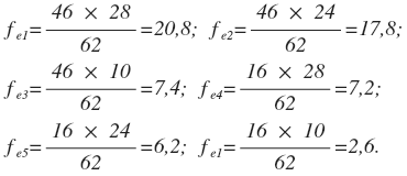
With the chi-square test, prior to the calculation of empirical value, it is necessary to calculate the expected frequencies (fe) in the cells typical for the total absence of relations between variables, and then to compare them with the available frequencies (fo). To do this, the marginal frequency in the column must be multiplied by the marginal frequency in the row and divided by the total number of observations, for each cell:

where MFR is the marginal frequency in the row, MFC is the marginal frequency in the column, N is the total number of observations.
For our example, the calculation of expected frequencies will be as follows:
For our example, the calculation of expected frequencies will be as follows:
Consequently, the table with the theoretical distribution characterized by the total absence of relations between variables will be as follows:
| Efficiency | Gender |
Total
|
|
Female |
Male |
||
| Satisfactory (with D and/or E) | 20,8 |
7,2 |
28 |
| Good or Excellent (no D/E, only B/C/A) | 17,8 |
6,2 |
24 |
| Excellent (only A) | 7,4 |
2,6 |
10 |
| Total | 46 |
16 |
62 |
If the difference between these frequencies and those obtained in the research are great enough, the alternative hypothesis will be adopted by, if not – the null hypothesis will be applied.
Difference value is determined with the help of special index / exponent, which is the empirical (or experimental) test value:
Difference value is determined with the help of special index / exponent, which is the empirical (or experimental) test value:
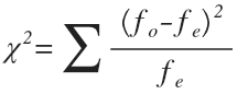
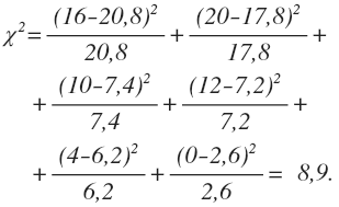
In our case, the empirical test value is equal to:
In addition to empirical value, most methods of statistical hypothesis testing involve the calculation of degrees of freedom (df), which are used in determining critical value, i.e. the value empirical value is compared with. This comparison estimates if empirical value is high enough (it must exceed critical value) to reject the null hypothesis and accept the alternative one. For the chi-square test df=(r-1)(c-1), where r is the number of rows in the table, c is the number of columns. Accordingly, in our case df=(3-1)(2-1)=2.
Step 5. All methods of statistical hypothesis testing involve the use of certain sample statistics distributions to determine critical value in each case study. Critical value, as well as empirical, is a special value that sets the limit which, when exceeded, states that there is a very low probability (this probability is equal to the alpha value) that the available results could be obtained due to random errors.
Step 5. All methods of statistical hypothesis testing involve the use of certain sample statistics distributions to determine critical value in each case study. Critical value, as well as empirical, is a special value that sets the limit which, when exceeded, states that there is a very low probability (this probability is equal to the alpha value) that the available results could be obtained due to random errors.
Chi-square distribution used for the analysis of contingency tables changes its form depending on the number of degrees of freedom. Consequently, the distribution of critical values changes as well (df is marked as k in the graph below):
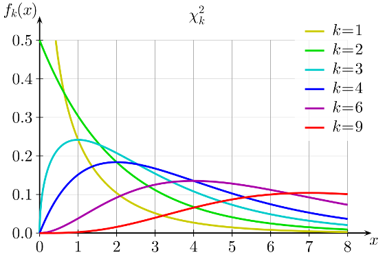
In each specific case, critical value itself is determined with the tables of critical values. With the chi-square test the table has two parameters – the number of degrees of freedom and the alpha level.
After critical value is determined, it must be compared with the empirical value – if critical value is higher, the null hypothesis is adopted (because the probability of obtaining results due to random errors is too high), if empirical value is higher, the alternative hypothesis is adopted.
For our example, the alpha value of 0.05 and df of 2 render the critical value of 5.99. Since the empirical value is higher than the critical value (8.9>5.99) the alternative hypothesis may be adopted. The probability of falsity in this case is 5%.
It is always important to remember that with statistical inference the researcher runs the risk of making a mistake, regardless of what hypothesis he/she adopts – null or alternative. Such errors are called statistical and are divided into two groups – type I and type II errors. With type I errors, the alternative hypothesis is adopted based on the sample data, while the null hypothesis is true for the population. With type II errors, the null hypothesis is adopted based on the sample data, while the alternative hypothesis is true for the population.
- default_titleХили Дж. Статистика. Социологические и маркетинговые исследования. - К.: ООО "ДиаСофтЮП"; СПб.: Питер, 2005. - 638 с.
- default_titleМалхотра Н. Маркетинговые исследования. - М: Вильямс, 2007. - 1200 с.
- default_titleField A. Discovering statistics using SPSS. - London, Thousand Oaks, New Delhi: Sage, 2009. - 822 p.
- Show More